Smooth and Conservative Upsampler

Apr 4, 2026 | Tech Robotics

Problem Statement

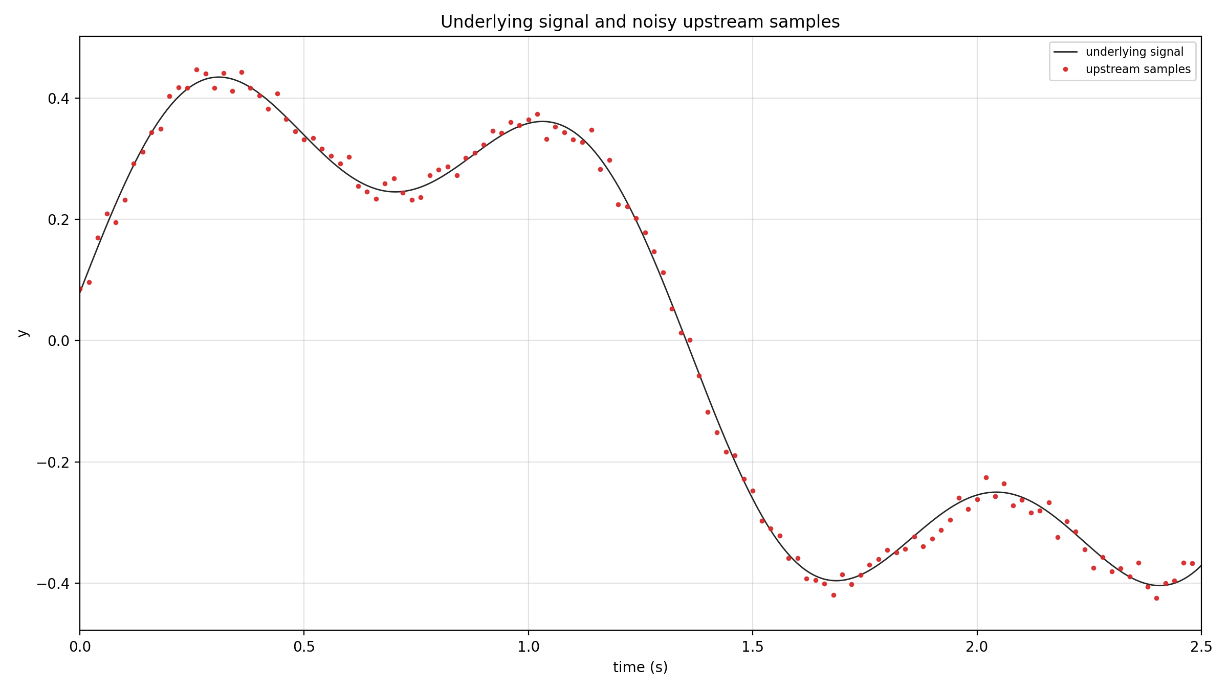
Upstream sends a time-ordered stream of samples $ (y_1, t_1), (y_2, t_2), \ldots, (y_n, t_n) $, with $ t_i $ strictly increasing, at a relatively low sample rate. The sample magnitude $y_i$ can be very unpredictable, with no obvious patterns. Our task as the middleman is to upsample this stream onto a much denser time grid for downstream to use in realtime. We want the high-rate trajectory to pass through, as much as possible, every received measurement and to be sufficiently smooth between them, i.e., smooth interpolation, not some free extrapolation of the future.

Key Ideas

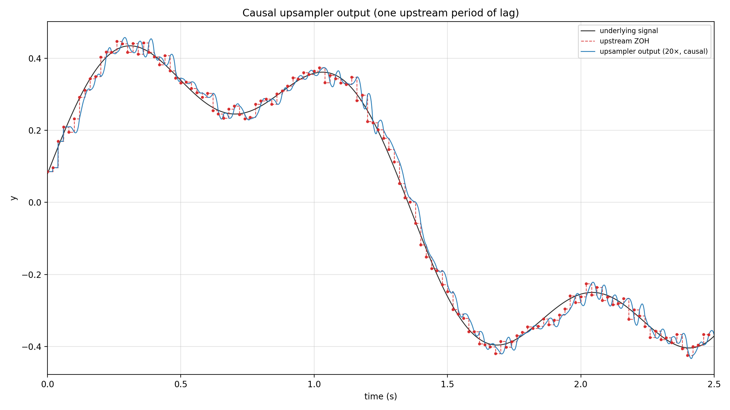
With no model of the future, a causal online method cannot output a polished value at the same time as the latest sample. The trade-off used here is a fixed delay of one sampling interval $ T $: whatever we emit to downstream is always computed from data that were already available at least one period ago. The processor buffers past samples, applies the local fit, and rolls forward, so downstream sees a stream that lags real time by $ T $, but each high-rate point is produced by the smooth polynomial interpolated from past samples rather than a raw zero-order hold or an extrapolation of the future.

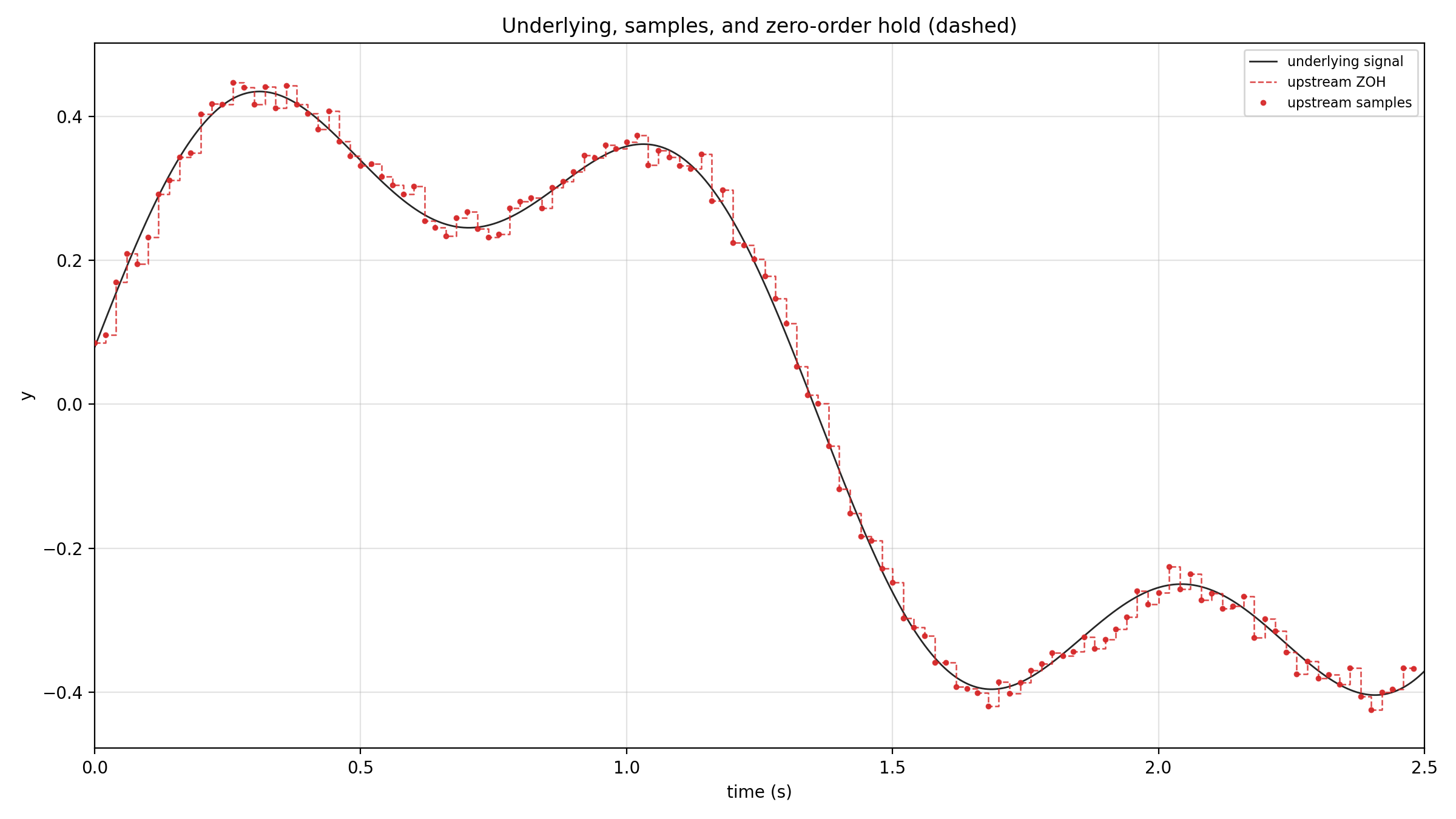
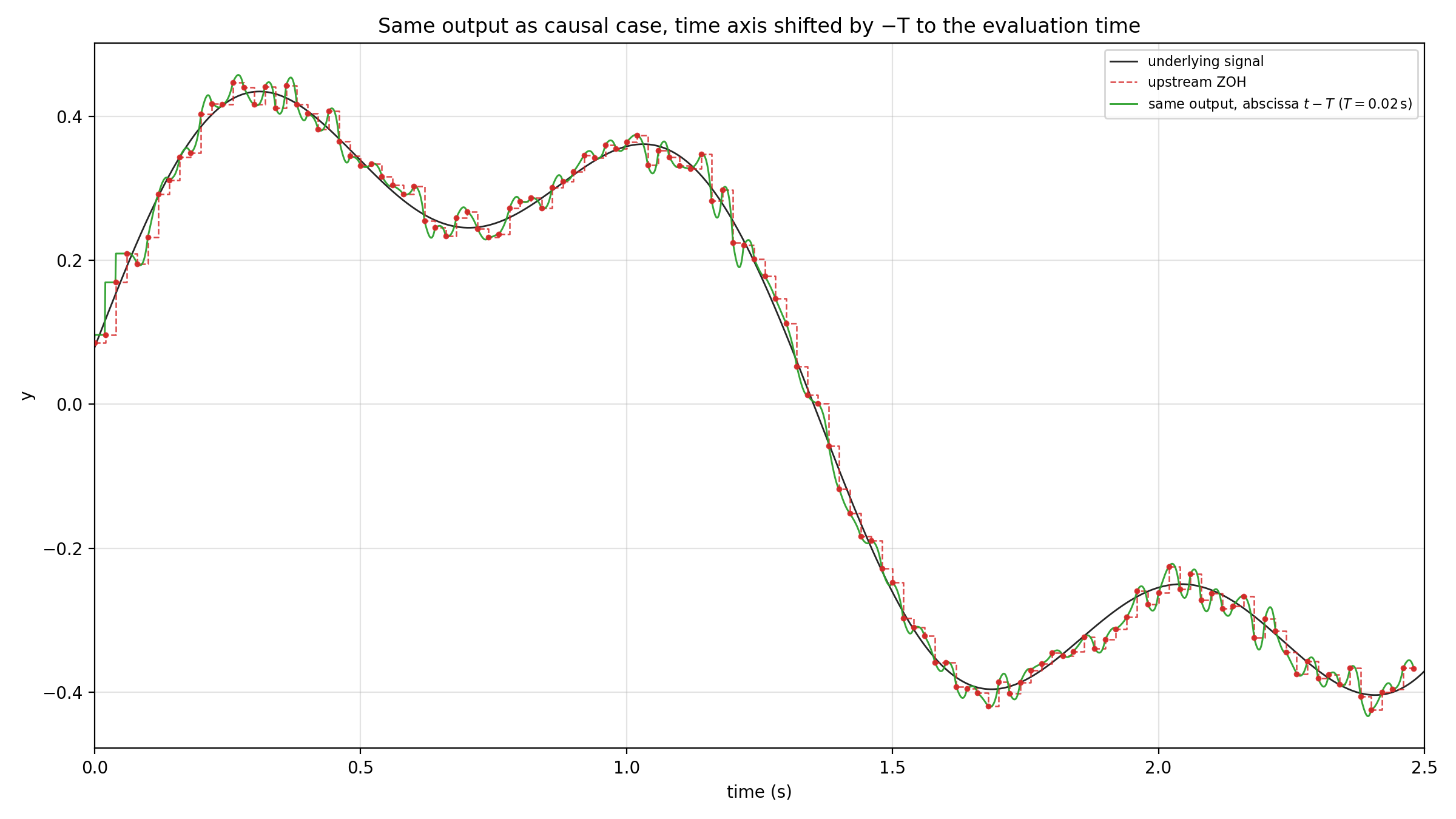
Concretely, we consider a 4-th degree polynomial to be sufficiently smooth for our purposes, hence we take five samples per fit. That is, we have a sliding window of five samples, with a delay of one sampling period $T$. Until the fifth sample has arrived at $t_5$, the high-rate output follows a zero-order hold on the last received value. After the fifth sample arrives at time $ t_5 $, consider wall-clock times $ t = t_5 + \tau $ with $ 0 \le \tau \lt T $ before the sixth sample at $ t_6 $. We fit $ y(t) $ through $ (y_i, t_i)_{i=1}^5 $, and assign $ \hat{y}(t_4 + \tau) $ to the output at time $ t_5 + \tau $, i.e., the same polynomial evaluated at the previous sample's time plus the same offset $ \tau $. Thus the output at $ t_5 + \tau $ is a smooth upsample, but lags the “natural” evaluation point by exactly one sampling period $ T $.

See also Savitzky-Golay filter for inspiration.

Local Polynomial Model

Inside one window, represent the fitted curve as a 4-th degree polynomial in time:

$$ y(t) = a_0 + a_1 t + a_2 t^2 + a_3 t^3 + a_4 t^4. $$

Collect the coefficients in a column vector $ \boldsymbol{\alpha} = \begin{bmatrix} a_0 & a_1 & a_2 & a_3 & a_4 \end{bmatrix}^{T} \in \mathbb{R}^5 $. For each sample $ (y_i, t_i) $ in the window,

$$ y_i = a_0 + a_1 t_i + a_2 t_i^2 + a_3 t_i^3 + a_4 t_i^4. $$

Denote the $ i $-th Vandermonde row, the power basis evaluated at $ t_i $, as:

$$ \boldsymbol{\tau}_i^{T} = \begin{bmatrix} 1 & t_i & t_i^2 & t_i^3 & t_i^4 \end{bmatrix}, $$

so that $ y_i = \boldsymbol{\tau}_i^{T} \boldsymbol{\alpha} $.

Stacking Equations

For $ i = 1, \ldots, 5 $ in the window, stack the measurements and rows:

$$ \mathbf{y} = \begin{bmatrix} y_1 \\ y_2 \\ y_3 \\ y_4 \\ y_5 \end{bmatrix}, \qquad \mathbf{T} = \begin{bmatrix} \boldsymbol{\tau}_1^{T} \\ \boldsymbol{\tau}_2^{T} \\ \boldsymbol{\tau}_3^{T} \\ \boldsymbol{\tau}_4^{T} \\ \boldsymbol{\tau}_5^{T} \end{bmatrix} = \begin{bmatrix} 1 & t_1 & t_1^2 & t_1^3 & t_1^4 \\ 1 & t_2 & t_2^2 & t_2^3 & t_2^4 \\ 1 & t_3 & t_3^2 & t_3^3 & t_3^4 \\ 1 & t_4 & t_4^2 & t_4^3 & t_4^4 \\ 1 & t_5 & t_5^2 & t_5^3 & t_5^4 \end{bmatrix}. $$

The five scalar equations $ y_i = \boldsymbol{\tau}_i^{T} \boldsymbol{\alpha} $ combine into the linear system

$$ \mathbf{y} = \mathbf{T} \, \boldsymbol{\alpha}, $$

with $ \mathbf{y} \in \mathbb{R}^5 $, $ \boldsymbol{\alpha} \in \mathbb{R}^5 $, and $ \mathbf{T} \in \mathbb{R}^{5 \times 5} $.

Solving for $ \boldsymbol{\alpha} $ and Evaluation

If $ t_1, \ldots, t_5 $ are distinct, the Vandermonde matrix $ \mathbf{T} $ is nonsingular; the coefficient vector is uniquely determined as

$$ \boldsymbol{\alpha} = \mathbf{T}^{-1} \mathbf{y}. $$

Note that in practical implementation, one can use QR or least squares to improve numerical stability; the solution agrees with the formula above whenever $ \mathbf{T} $ is invertible. Given $ \boldsymbol{\alpha} $, the fitted polynomial is $ y(t) = \sum_{k=0}^{4} a_k t^k $. Its value at any time $ t $ in the window on a denser grid is

$$ \hat{y}(t) = \begin{bmatrix} 1 & t & t^2 & t^3 & t^4 \end{bmatrix} \, \boldsymbol{\alpha} = \boldsymbol{\tau}^{T}(t) \, \boldsymbol{\alpha}. $$

Sliding a five-sample window along the stream of data, repeating this fit, and outputting the interpolated value at each time step with one sampling period delay, we address the challenge in the problem statement with the ideas purposed above.

Notes

Design Considerations and Limitations

We choose a quartic polynomial because within each window the acceleration is smooth and the jerk varies linearly in time, which is usually “smooth enough” for many control pipelines. Algebraically, five samples and five coefficients give a square Vandermonde system - invert it once per window and the cost stays small. The downside is visible in the plots below, local polynomial interpolation can overshoot between samples, so this is not a globally optimal smoother. It is only a simple, fast, and relatively conservative one.

Extensions

Richer formulations can impose hard or soft limits on overshoot, speed, acceleration, jerk, and so on - typically via convex or nonlinear optimization. That often tracks the underlying signal better but adds latency and CPU cost per step. Recursive estimators (Kalman-family filters) help when the signal obeys a useful state-space model; with largely patternless upstream data, tuning and performance gains are harder to rely on. In practice it is a balance among latency, compute, smoothness, and fidelity.

Demonstrations

Underlying Signal, Measured, ZOH

Upsampled, Shifted Upsampled

Animated ZOH vs. Smooth Upsampling

Implementation

See below for code generating the above demonstrations.